Using ABS structures
Loading the package will lazily load a number of structures, a full list is available in the reference
glimpse(anzsco2009)
#> Rows: 1,180
#> Columns: 11
#> $ anzsco_major_code      <chr> "1", "1", "1", "1", "1", "1", "1", "1", "1", "1…
#> $ anzsco_major           <chr> "Managers", "Managers", "Managers", "Managers",…
#> $ anzsco_submajor_code   <chr> "10", "11", "11", "11", "11", "11", "11", "11",…
#> $ anzsco_submajor        <chr> "Managers, nfd", "Chief Executives, General Man…
#> $ anzsco_minor_code      <chr> "100", "110", "111", "111", "111", "111", "111"…
#> $ anzsco_minor           <chr> "Managers, nfd", "Chief Executives, General Man…
#> $ anzsco_unit_code       <chr> "1000", "1100", "1110", "1111", "1112", "1112",…
#> $ anzsco_unit            <chr> "Managers, nfd", "Chief Executives, General Man…
#> $ anzsco_occupation_code <chr> "100000", "110000", "111000", "111111", "111211…
#> $ anzsco_occupation      <chr> "Managers, nfd", "Chief Executives, General Man…
#> $ skill_level            <chr> NA, NA, NA, "1", "1", "1", "1", "1", "1", NA, N…
glimpse(anzsic2006)
#> Rows: 506
#> Columns: 8
#> $ anzsic_division_code    <chr> "A", "A", "A", "A", "A", "A", "A", "A", "A", "…
#> $ anzsic_division         <chr> "Agriculture, Forestry and Fishing", "Agricult…
#> $ anzsic_subdivision_code <chr> "1", "1", "1", "1", "1", "1", "1", "1", "1", "…
#> $ anzsic_subdivision      <chr> "Agriculture", "Agriculture", "Agriculture", "…
#> $ anzsic_group_code       <chr> "11", "11", "11", "11", "11", "12", "12", "12"…
#> $ anzsic_group            <chr> "Nursery and Floriculture Production", "Nurser…
#> $ anzsic_class_code       <chr> "111", "112", "113", "114", "115", "121", "122…
#> $ anzsic_class            <chr> "Nursery Production (Under Cover)", "Nursery P…
glimpse(asced_foe2001)
#> Rows: 439
#> Columns: 6
#> $ aced_foe_broad_code    <chr> "01", "01", "01", "01", "01", "01", "01", "01",…
#> $ aced_foe_broad         <chr> "Natural and Physical Sciences", "Natural and P…
#> $ aced_foe_narrow_code   <chr> "0100", "0101", "0101", "0101", "0101", "0103",…
#> $ aced_foe_narrow        <chr> "Natural and Physical Sciences, nfd", "Mathemat…
#> $ aced_foe_detailed_code <chr> "010000", "010100", "010101", "010103", "010199…
#> $ aced_foe_detailed      <chr> "Natural and Physical Sciences, nfd", "Mathemat…
glimpse(asced_qual2001)
#> Rows: 64
#> Columns: 6
#> $ aced_qual_broad_code    <chr> "1", "1", "1", "1", "1", "1", "1", "1", "1", "…
#> $ aced_qual_broad         <chr> "Postgraduate Degree Level", "Postgraduate Deg…
#> $ aced_qual_narrow_code   <chr> "11", "11", "11", "11", "11", "11", "12", "12"…
#> $ aced_qual_narrow        <chr> "Doctoral Degree Level", "Doctoral Degree Leve…
#> $ aced_qual_detailed_code <chr> "111", "112", "113", "114", "115", "116", "121…
#> $ aced_qual_detailed      <chr> "Higher Doctorate", "Doctorate by Research", "…
Objects stored in the absmapsdata package can be accessed with the read_absmap function:
library(sf) # loaded to handle sf objects
#> Linking to GEOS 3.10.2, GDAL 3.4.2, PROJ 8.2.1; sf_use_s2() is TRUE
read_absmap("sa42016")
#> Simple feature collection with 107 features and 9 fields (with 18 geometries empty)
#> Geometry type: MULTIPOLYGON
#> Dimension:     XY
#> Bounding box:  xmin: 96.81695 ymin: -43.74048 xmax: 167.9969 ymax: -9.219937
#> Geodetic CRS:  WGS 84
#> First 10 features:
#>    sa4_code_2016               sa4_name_2016 gcc_code_2016  gcc_name_2016
#> 1            101              Capital Region         1RNSW    Rest of NSW
#> 2            102               Central Coast         1GSYD Greater Sydney
#> 3            103                Central West         1RNSW    Rest of NSW
#> 4            104     Coffs Harbour - Grafton         1RNSW    Rest of NSW
#> 5            105          Far West and Orana         1RNSW    Rest of NSW
#> 6            106 Hunter Valley exc Newcastle         1RNSW    Rest of NSW
#> 7            107                   Illawarra         1RNSW    Rest of NSW
#> 8            108             Mid North Coast         1RNSW    Rest of NSW
#> 9            109                      Murray         1RNSW    Rest of NSW
#> 10           110  New England and North West         1RNSW    Rest of NSW
#>    state_code_2016 state_name_2016 areasqkm_2016 cent_long  cent_lat
#> 1                1 New South Wales     51895.563  149.2450 -35.56480
#> 2                1 New South Wales      1681.072  151.2855 -33.30797
#> 3                1 New South Wales     70297.060  148.3558 -33.21697
#> 4                1 New South Wales     13229.758  152.7739 -29.81603
#> 5                1 New South Wales    339363.693  145.0269 -30.98611
#> 6                1 New South Wales     21491.291  150.9849 -32.35481
#> 7                1 New South Wales      1538.919  150.7711 -34.43464
#> 8                1 New South Wales     18851.500  152.3410 -31.56476
#> 9                1 New South Wales     97797.675  144.0434 -34.42275
#> 10               1 New South Wales     99145.916  150.7019 -30.06335
#>                          geometry
#> 1  MULTIPOLYGON (((150.3113 -3...
#> 2  MULTIPOLYGON (((151.315 -33...
#> 3  MULTIPOLYGON (((150.6107 -3...
#> 4  MULTIPOLYGON (((153.2785 -2...
#> 5  MULTIPOLYGON (((150.1106 -3...
#> 6  MULTIPOLYGON (((152.3165 -3...
#> 7  MULTIPOLYGON (((150.8783 -3...
#> 8  MULTIPOLYGON (((159.0686 -3...
#> 9  MULTIPOLYGON (((147.6165 -3...
#> 10 MULTIPOLYGON (((152.4876 -2...
Converting state names and abbreviations
The clean_state() function makes it easy to wrangle vectors of State names and abbreviations - which might be in different forms and possibly misspelled.
Let’s start with a character vector that includes some misspelled state names, some correctly spelled state names, as well as some abbreviations both malformed and correctly formed.
x <- c("western Straya", "w. A ", "new soth wailes", "SA", "tazz", "Victoria",
       "northn territy")
To convert this character vector to a vector of abbreviations for State names, use clean_state():
clean_state(x)
#> [1] "WA"  "WA"  "NSW" "SA"  "Tas" "Vic" "NT"
If you want full names for the states rather than abbreviations:
clean_state(x, to = "state_name")
#> [1] "Western Australia"  "Western Australia"  "New South Wales"
#> [4] "South Australia"    "Tasmania"           "Victoria"
#> [7] "Northern Territory"
By default, clean_state() uses fuzzy or approximate string matching to match the elements in your character vector to state names/abbreviations. If you only want to permit exact matching, you can disable fuzzy matching. This means you will never get false matches, but you will also fail to match misspelled state names or malformed abbreviations; you’ll get an NA if no match can be found.
 clean_state(x, fuzzy_match = FALSE)
#> [1] NA    NA    NA    "SA"  NA    "Vic" NA
If your data is in a data frame, clean_state() works well within a dplyr::mutate() call:
 x_df <- data.frame(state = x, stringsAsFactors = FALSE)

library(dplyr)
 x_df %>%
   mutate(state_abbr = clean_state(state))
#>             state state_abbr
#> 1  western Straya         WA
#> 2           w. A          WA
#> 3 new soth wailes        NSW
#> 4              SA         SA
#> 5            tazz        Tas
#> 6        Victoria        Vic
#> 7  northn territy         NT
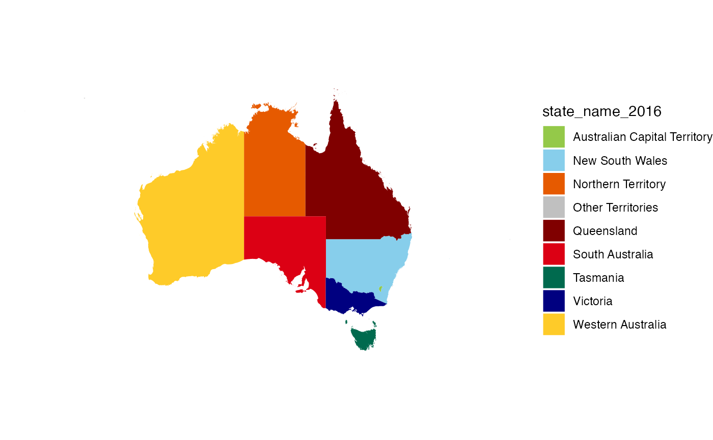
The function clean_state can also return an ‘unofficial’ state/territory colour for use in charts.
clean_state("Queensland", to = "colour")
#> [1] "#800000"
The palette palette_state_name_2016 can be used in ggplot2 for the unofficial colours of states.
read_absmap("state2016") %>%
    ggplot() +
    geom_sf(aes(fill = state_name_2016), colour = NA) +
    scale_fill_manual(values = palette_state_name_2016) +
    theme_void()
Australian public holidays
This package includes the auholidays dataset from the Australian Public Holidays Dates Machine Readable Dataset as well as a helper function is_holiday:
str(auholidays)
#> tibble [879 × 3] (S3: tbl_df/tbl/data.frame)
#>  $ Date        : Date[1:879], format: "2021-01-01" "2021-01-26" ...
#>  $ Name        : chr [1:879] "New Year's Day" "Australia Day" "Canberra Day" "Good Friday" ...
#>  $ Jurisdiction: chr [1:879] "ACT" "ACT" "ACT" "ACT" ...


is_holiday('2020-01-01')
#> [1] TRUE
is_holiday('2019-05-27', jurisdictions = c('ACT', 'TAS'))
#> [1] TRUE

h_df <- data.frame(dates = c('2020-01-01', '2020-01-10'))

h_df %>%
  mutate(IsHoliday = is_holiday(dates))
#>        dates IsHoliday
#> 1 2020-01-01      TRUE
#> 2 2020-01-10     FALSE
Parsing income ranges
The parse_income_range function provides some tools for extracting numbers from income ranges commonly used in Australian data. For example:
parse_income_range("$1-$199 ($1-$10,399)", limit = "lower")
#> [1] 1
parse_income_range("$1-$199 ($1-$10,399)", limit = "upper")
#> [1] 199
parse_income_range("$1-$199 ($1-$10,399)", limit = "mid")
#> [1] 100

parse_income_range("e. $180,001 or more", limit = "upper")
#> [1] Inf
parse_income_range("e. $180,001 or more", limit = "upper", max_income = 300e3)
#> [1] 3e+05


parse_income_range("Nil income")
#> [1] 0
parse_income_range("Negative income")
#> [1] 0
parse_income_range("Negative income", negative_as_zero = FALSE)
#> [1] NA


tibble(income_range = c("Negative income",
                        "Nil income",
                        "$1,500-$1,749 ($78,000-$90,999)",
                        "$1,750-$1,999 ($91,000-$103,999)",
                        "$2,000-$2,999 ($104,000-$155,999)",
                        "$3,000 or more ($156,000 or more)")) %>%
  mutate(lower = parse_income_range(income_range),
         mid   = parse_income_range(income_range, limit = "mid"),
         upper = parse_income_range(income_range, limit = "upper"))
#> # A tibble: 6 × 4
#>   income_range                      lower   mid upper
#>   <chr>                             <dbl> <dbl> <dbl>
#> 1 Negative income                       0     0     0
#> 2 Nil income                            0     0     0
#> 3 $1,500-$1,749 ($78,000-$90,999)    1500  1625  1749
#> 4 $1,750-$1,999 ($91,000-$103,999)   1750  1875  1999
#> 5 $2,000-$2,999 ($104,000-$155,999)  2000  2500  2999
#> 6 $3,000 or more ($156,000 or more)  3000   Inf   Inf